
Expectation Maximization Algorithm and Gaussian Mixtures
The EM algorithm is a powerful iterative method for finding maximum likelihood estimates in statistical models with “latent variables” or missing data. It was first proposed by Dempster, Laird, and Rubin (1977), and since then it has been a common tool in machine learning models.
Actually, it is simple, but tricky. The core idea is to iteratively alternate between two steps until convergence:
- Expectation (E) step: Estimate the missing data given the observed data and current parameter estimates.
- Maximization (M) step: Update the parameters to maximize the likelihood, treating the estimated missing data as if it were observed.
Eventually (hopefully) the algorithm converges. This is particularly useful for Gaussian mixture models.
A labor market with hidden types
Say we observe labor market data with log wages and we suspect it is actually composed of two types of workers: low types and high types. However, we do not observe the worker type, we only observe the social identifier and their payment. Assume just one firm with a constant rent-sharing policy — no matter the type of the worker, their wage in expectation is simply the average value of their types.
This concept of discrete worker types is not too far away from reality. Individuals are constantly accumulating human capital, either through school or work experience. You can think of this concept as broad categories of human capital accumulation.
Let us construct this labor market:
library(tidyverse)

set.seed(123)
n <- 10000
true_means <- c(2, 3)
true_sds <- c(0.5, 0.5)
true_weights <- c(0.6, 0.4)

lmarket <- tibble(
  worker_id = 1:n,
  type = c(rep(1, n * true_weights[1]), rep(2, n * true_weights[2])),
  log_wage = c(
    rnorm(n * true_weights[1], true_means[1], true_sds[1]),
    rnorm(n * true_weights[2], true_means[2], true_sds[2])
  )
) |>
  mutate(log_wage = log_wage - min(log_wage) + 1)
Here I generated 10,000 workers. Every time a worker is hired, they draw their log wage from a normal distribution specific to their type.
Because I want strictly positive log wages, after the draw, I subtract the minimum observed wage and add one unit. This distorts the moments, so let us recheck:
lmarket |>
  group_by(type) |>
  summarize(mean_wage = mean(log_wage), sd_wage = sd(log_wage))
#> # A tibble: 2 x 3
#>    type mean_wage sd_wage
#>   <dbl>     <dbl>   <dbl>
#> 1     1      2.63   0.497
#> 2     2      3.62   0.503
So worker $i$, if they are high types, draws from $w_i \sim \mathcal{N}(3.62, 0.50)$, with probability $P_{high} = 0.40$. Low types draw from $w_i \sim \mathcal{N}(2.63, 0.50)$, with $P_{low} = 0.60$.
We can formally write this mixture as:
\[f(w_i; \mu, \sigma, \pi) = \sum^2_{k = 1} \pi_k \mathcal{N}(w_i; \mu_k, \sigma_k)\]The histogram
ggplot(lmarket, aes(x = log_wage)) +
  geom_histogram(bins = 80, fill = "#2d2d2d", alpha = 0.8, color = "white", linewidth = 0.2) +
  labs(x = "Log Wage", y = "Count", title = "Distribution of Log Wages") +
  theme_minimal(base_size = 14) +
  theme(
    plot.title = element_text(face = "bold", color = "#2d2d2d"),
    panel.grid.minor = element_blank()
  )
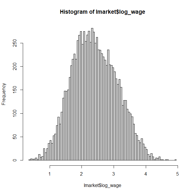
Notice how we can barely see the mixture components in this histogram. In real-world data, wages are all over the place the same way. However, if we are to believe a particular human capital amount has a direct effect on potential income, it is hard to conclude all workers draw from a single distribution. There must be “hidden” distributions blended together. So how do we extract them?
The EM algorithm
The first step is to guess the initial moments and priors. For the guess, we can use a simple k-means routine to slice the data. Since we know this mixture has two components, we slice the data in 2 parts.
# Initial guess via k-means
initial_guess <- kmeans(lmarket$log_wage, centers = 2, nstart = 25)$cluster

mu1 <- mean(lmarket$log_wage[initial_guess == 1])
mu2 <- mean(lmarket$log_wage[initial_guess == 2])
sigma1 <- sd(lmarket$log_wage[initial_guess == 1])
sigma2 <- sd(lmarket$log_wage[initial_guess == 2])
pi1 <- mean(initial_guess == 1)
pi2 <- mean(initial_guess == 2)
We need to find the observed-data log-likelihood, which for a mixture model is:
\[\ell = \sum_i \log \left( \sum_k \pi_k \mathcal{N}(w_i; \mu_k, \sigma_k) \right)\]Note the log of the sum — this is what makes direct maximization difficult and motivates the EM approach.
# Helper: sum only finite values (avoids log(0) issues)
sum_finite <- function(x) sum(x[is.finite(x)])

# Starting log-likelihood (observed-data version)
L <- c(-Inf, sum(log(pi1 * dnorm(lmarket$log_wage, mu1, sigma1) +
                      pi2 * dnorm(lmarket$log_wage, mu2, sigma2))))
Now we iterate between E and M steps until convergence:
current_iter <- 2
max_iter <- 500

while (abs(L[current_iter] - L[current_iter - 1]) >= 1e-8 && current_iter < max_iter) {
  # E step: compute posterior probabilities
  comp1 <- pi1 * dnorm(lmarket$log_wage, mu1, sigma1)
  comp2 <- pi2 * dnorm(lmarket$log_wage, mu2, sigma2)
  comp_sum <- comp1 + comp2

  p1 <- comp1 / comp_sum
  p2 <- comp2 / comp_sum

  # M step: update parameters
  pi1 <- sum_finite(p1) / length(lmarket$log_wage)
  pi2 <- sum_finite(p2) / length(lmarket$log_wage)

  mu1 <- sum_finite(p1 * lmarket$log_wage) / sum_finite(p1)
  mu2 <- sum_finite(p2 * lmarket$log_wage) / sum_finite(p2)

  sigma1 <- sqrt(sum_finite(p1 * (lmarket$log_wage - mu1)^2) / sum_finite(p1))
  sigma2 <- sqrt(sum_finite(p2 * (lmarket$log_wage - mu2)^2) / sum_finite(p2))

  # Recompute log-likelihood with UPDATED parameters
  current_iter <- current_iter + 1
  L[current_iter] <- sum(log(pi1 * dnorm(lmarket$log_wage, mu1, sigma1) +
                              pi2 * dnorm(lmarket$log_wage, mu2, sigma2)))
}
In the E step, we compute the likelihood of each data point under each Gaussian component, weighted by their prior probabilities. Then we normalize to get posterior probabilities for each data point.
In the M step, we use these posteriors to update the mixing proportions, means, and standard deviations. Crucially, we recompute the log-likelihood using the updated parameters — this ensures the convergence criterion correctly reflects the improvement from the M step. The EM algorithm guarantees monotone ascent: $\ell(\theta^{(t+1)}) \geq \ell(\theta^{(t)})$.
Results
cat(sprintf("Converged in %d iterations\n", current_iter - 2))
cat(sprintf("  Component 1: mu = %.3f, sigma = %.3f, pi = %.3f\n", mu1, sigma1, pi1))
cat(sprintf("  Component 2: mu = %.3f, sigma = %.3f, pi = %.3f\n", mu2, sigma2, pi2))
#> Converged in 498 iterations
#>   Component 1: mu = 2.654, sigma = 0.498, pi = 0.614
#>   Component 2: mu = 3.641, sigma = 0.502, pi = 0.386
The estimated means, standard deviations, and mixing proportions are very close to the true values ($\mu_1 \approx 2.63$, $\mu_2 \approx 3.62$, $\pi_1 \approx 0.60$, $\pi_2 \approx 0.40$). We can visualize the recovered components overlaid on the histogram:
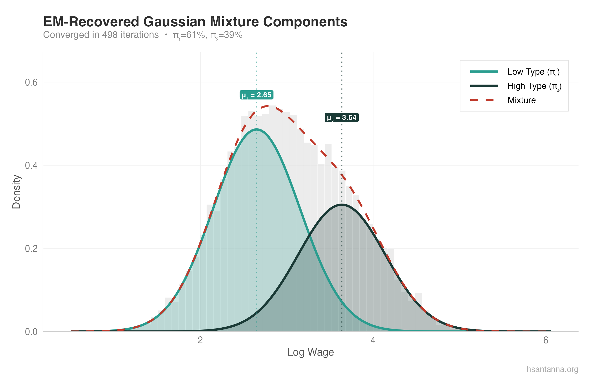
The two Gaussian components (teal and dark teal) are clearly separated, and their weighted sum (dashed red) closely matches the empirical density.
What about model selection?
But wait, how do we know how many mixture components there are? This is a very important question. Assuming too few components will group together observations that are in fact distinct. Too many, and similar observations will end up in different components.
What happens if we assume 3 worker types instead of 2? You can quickly extend the algorithm with a third component. Doing so yields a tiny third component ($\hat{\pi}_3 \approx 0.018$) that the algorithm struggles to fit — a clear sign of overfitting.
So how to choose the most appropriate number of worker types? The answer lies in systematic model comparison. Test multiple settings, observe the patterns. Are we far from proper economic theory? Is it parsimonious enough to provide good intuition? Information criteria like AIC or BIC can guide you — they penalize model complexity, helping balance fit against overfitting.