
So, what is bunching?
Here I will explain the basic concepts of bunching as a causal inference method. The full replication code is at the bottom of this post and also available on GitHub.
library(tidyverse)
library(ggdag)
library(AER)

set.seed(20240804)
Constructing the data
We need a data generating process where an unobserved confounder $\eta$ affects both the treatment (cigarettes) and the outcome (birth weight), while a covariate (education) is also observed.
n <- 5000

# Covariates
educ <- sample(6:16, n, replace = TRUE)
eta <- rnorm(n)

# Latent smoking propensity (running variable)
cigs_star <- 20 - 1.5 * educ + 5 * eta + rnorm(n, 0, 3)

# Observed cigarettes: censored at zero
cigs <- pmax(0, round(cigs_star))

# Birth weight: affected by cigs, education, AND eta
bw <- 3000 - 20 * cigs + 15 * educ - 10 * eta + rnorm(n, 0, 100)

data <- tibble(bw = bw, cigs = cigs, educ = educ)
Notice the key feature: $\eta$ directly affects both cigs_star (smoking propensity) and bw (birth weight). This is the unobserved confounder that will bias naive estimates.
The naive approach
Imagine that you are interested in the causal effect of smoking on birth weights. Say you observe a covariate, mom’s education, and you are willing to control for that.
Okay, that sounds good. Perhaps people with more education are more inclined to not smoke, have better healthcare, etc. For simplicity, you could impose a linear model:
\[y_i = \beta X_i + \gamma Z_i + \varepsilon_i\]Where $y_i$ is the birth weight of baby $i$, $X_i$ is the number of cigarettes smoked by baby $i$’s mom, and $Z_i$ is the mom’s education. $\varepsilon_i$ is a random shock where $\mathbb{E}(\varepsilon \mid X, Z) = 0$.
Say you have these variables in a neat dataset, so you run the regression:
naive_model <- lm(bw ~ cigs + educ, data = data)
summary(naive_model)
Do you notice something weird about this regression? Can you say that for every cigarette smoked per day, the baby loses about 40 grams?
Probably not!
This is why it is important to always have economic intuition as your sanity check.
The hint lies on the educ coefficient. It is either wrong-signed or insignificant — it implies babies are worse off (or no better off) as we increase the mom’s education level.
What is happening here then?
The problem lies in what we do not observe. What if there is a variable, unobserved $\eta$, which influences not only birth weights directly but also the propensity to smoke?
Let us make a DAG representing this using ggdag:
dag <- dagify(
  bw ~ cigs + educ + eta,
  cigs ~ educ + eta,
  labels = c(
    "bw" = "Birth Weight",
    "cigs" = "Cigarettes",
    "educ" = "Education",
    "eta" = "Unobserved\nFactors"
  ),
  exposure = "cigs",
  outcome = "bw"
)

ggdag_dseparated(dag, "eta", text = FALSE, use_labels = "label") +
  theme_dag_blank() +
  theme(legend.position = "none")
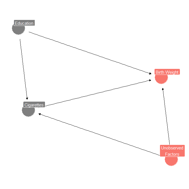
Notice there are 3 causal paths to birth weights. The first is a direct path from education, another from $\eta$, and another where cigarettes act as a mediator variable.
If that is the case, not only are we incorrectly estimating the causal relationship between cigarettes and birth weights, we are probably messing with the education path too.
Enter bunching
So how to solve this problem? This is where bunching comes into play.
The key assumption: there is a proxy relationship between smoking and covariates. Individuals have a propensity to smoke, like a utility function. Some maximize this utility by smoking heavily. Others are very averse — they would pay not to smoke. And then there are the marginally inclined — they would smoke given a chance but are slightly better off not smoking.
The implication is interesting because we partially observe this mechanism. We only see individuals who are positively inclined to smoke! There is no way to observe negative cigarette consumption.
What happens if we plot the relationship?
ggplot(data, aes(x = cigs, y = bw)) +
  geom_point(aes(color = cigs), alpha = 0.6, size = 2) +
  geom_smooth(method = "lm", color = "#2a9d8f", fill = "#2a9d8f", alpha = 0.2) +
  scale_color_gradient(low = "#7ecfc4", high = "#2d2d2d") +
  labs(
    title = "Cigarette Consumption vs. Birth Weight",
    x = "Cigarettes Smoked per Day",
    y = "Birth Weight (grams)",
    color = "Cigarettes\nper Day"
  ) +
  theme_minimal(base_size = 14) +
  theme(
    plot.title = element_text(face = "bold", color = "#2d2d2d"),
    panel.grid.minor = element_blank()
  )
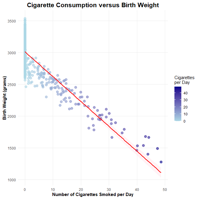
What catches your eye? Notice that this is a pretty linear relationship, until it is not: as soon as we reach 0 cigarettes, we observe a bunching pattern of birth weights.
The right question is: why are there so many data points accumulated at zero? This is the puzzle we must solve.
The running variable
The answer: there is a variable we do not observe that “runs” in that relationship continuously and accepts negative values of cigarettes. This variable is affected by both observables (education) and unobservables ($\eta$). If we could capture this variable, we could isolate the relationship between cigarettes and birth weights without the confounding $\eta$ factor.
Formally:
\[X = \max(0, X^*)\]That is, $X$, the observed variable, is a proxy for $X^*$, the running variable that is continuous in zero and can assume negative values.
If we assume linearity:
\[Y = \beta X + Z'\gamma + \delta \eta + \varepsilon\] \[X^* = Z'\pi + \eta\]The running variable of cigarettes is a linear function of the observable (education) and the unobservable ($\eta$). Our objective is to recover $X^*$ and use it as a proxy for $\eta$. If we can, we bypass the confounding.
Combining these equations:
\[\mathbb{E}(Y \mid X,Z) = X\beta + Z'(\gamma - \pi\delta) + \delta\left(X + \mathbb{E}(X^* \mid X^* \leq 0, Z)\cdot\mathbb{1}(X = 0)\right)\]The trick is that we impute $\mathbb{E}(X^* \mid X^* \leq 0, Z)\cdot\mathbb{1}(X = 0)$ as a proxy for when X becomes 0 — we now “observe” negative values for smoking cigarettes. This accounts for the unobservable confounder.
The Tobit approach
Since our data is censored at zero, we assume linearity and normality of the latent error: $\eta \sim \mathcal{N}(0, \sigma^2)$. This allows us to use a Tobit model to recover the truncated conditional expectation $\mathbb{E}(X^* \mid X^* \leq 0, Z)$:
# Fit Tobit model
tobit_model <- tobit(cigs ~ educ, data = data, left = 0)

# Extract Tobit parameters
sigma_hat <- tobit_model$scale
xb <- predict(tobit_model, type = "lp")  # linear predictor: Z'pi_hat

# Compute E(X* | X* <= 0, Z) using the inverse Mills ratio
# For truncation from above at 0: E(X*|X*<=0) = Z'pi - sigma * phi(-Z'pi/sigma) / Phi(-Z'pi/sigma)
mills <- dnorm(-xb / sigma_hat) / pnorm(-xb / sigma_hat)
trunc_exp <- xb - sigma_hat * mills

# Control function: truncated expectation at the bunching point, zero for smokers
data <- data |>
  mutate(cf_imput = ifelse(cigs == 0, trunc_exp, 0))
The key step is the inverse Mills ratio correction. The linear predictor $Z’\hat{\pi}$ alone is not $\mathbb{E}(X^* \mid X^* \leq 0, Z)$ — we must account for the truncation. For a normal distribution truncated from above at zero, this expectation is $Z’\hat{\pi} - \hat{\sigma} \cdot \frac{\phi(-Z’\hat{\pi}/\hat{\sigma})}{\Phi(-Z’\hat{\pi}/\hat{\sigma})}$, where $\phi$ and $\Phi$ are the standard normal PDF and CDF.
Now fit the full model with the imputed control function:
cf_model <- lm(bw ~ cigs + educ + cf_imput, data = data)
summary(cf_model)
The coefficient on cigs should now be close to the true value of $\beta = -20$. Compare this with the naive OLS, which was biased toward $-40$. The control function method successfully removed the endogeneity from average smoked cigarettes per day.
Where is the randomness?
Causal experiments usually rely on random shocks or exogenous “manipulation” to build identification. But here there is no randomness, right? Individuals bunched at zero simply because they cannot smoke less than zero. Their propensity to smoke is hardwired in their utility function.
I think the correct way to think about this is to understand why we require randomness in the first place. We need randomness to ensure unobservables are not affecting the treatment effect. In bunching, we exploit the bunched values to reach the unobservable confounder and ultimately control for it.
Further reading
Bunching can definitely increase in complexity. We do not need to assume normality or a linear model. We do not even need parametrization! For a deeper overview, I suggest reading Bertanha, McCallum, and Seegert (2024) and the original Caetano (2015).