
Quick Start to Doubly Robust Estimators
Here, I will provide a simple explanation on doubly robust estimators using R’s tidyverse. This post is heavily inspired by Matheus Facure’s Causal Inference for the Brave and True. There you can find comprehensive tutorials of many causal inference models in Python.
In a first introduction to causal inference, we learn about linear estimators and propensity score weighting methods to estimate the average treatment effect conditional on covariates.
However, covariates are the main source of confounding in causal inference settings, so we should ask: which method should we use? In fact, we can combine both to achieve consistent estimation even when one of the models is misspecified!
Setting up the data
Let us imagine we are investigating the causal relationship between income and a government training program in which individuals may or may not participate.
First, we create a very simple static “labor market”. Assume 10,000 workers for whom we observe two variables, X1 and X2.
library(tidyverse)
library(fixest)

set.seed(123)

n <- 10000

# Generate covariates
X1 <- rnorm(n)
X2 <- rnorm(n)
For the sake of simplicity, X1 and X2 are standard normal distributions. We can assume there is a function that maps these draws to real-world data variables — for example, education and work experience.
Treatment assignment
Let us now create a treatment variable. In several cases dealing with real-world data, where there is no randomized experiment, assignment to treatment is actually correlated to certain variables in a functional form we may not know.
The key identifying assumption in this exercise is unconfoundedness (also called selection on observables): conditional on X1 and X2, treatment assignment is independent of potential outcomes:
\[\left(Y(1), Y(0)\right) \perp D \mid X_1, X_2\]This means that, after conditioning on the covariates, there are no remaining unobserved factors that simultaneously affect both treatment and outcomes. We also require overlap: $0 < P(D = 1 \mid X) < 1$, ensuring that every type of individual has a positive probability of being treated or untreated.
In this labor market example, individuals may observe the opportunity to enter the program but some of them are inclined to not participate given they accumulated enough human capital.
# Generate treatment via logistic model
ps_true <- plogis(-1 - 0.5 * X1 - 0.5 * X2)
treat <- rbinom(n, 1, ps_true)
In this case, ps_true represents a logistic function that maps the relationship of X1 and X2 to the treatment variable. The assignment to treatment is generated by a binomial distribution that observes these propensity scores and draws a success (participated in the training program) or a failure (refused to participate). Note that the relationship is negative: higher values of human capital increase the likelihood of no participation.
The naive ATE
Can we simply do an ATE calculation in this case? Let us finish constructing the data by creating the income variable Y and calculate the classical ATE.
# Treatment effect
tau <- 0.5

# Generate the data
df <- tibble(
  id = 1:n,
  X1 = X1,
  X2 = X2,
  treat = treat,
  Y = tau * treat + 0.25 * X1 + 0.25 * X2 + rnorm(n, 0, 0.5)
)

# Naive ATE calculation
naive_ATE <- df |>
  group_by(treat) |>
  summarize(meanY = mean(Y)) |>
  summarize(ATE = diff(meanY)) |>
  pull()

naive_ATE
#> [1] 0.2863138
The true treatment effect of the training program is $\tau = 0.5$. However, when calculating the ATE by simply finding average outcomes from treatment and control group, the estimate is biased downward by nearly half.
This can also be verified using an incomplete linear model, where covariates are not included:
# Naive linear estimator
feols(Y ~ treat, data = df)
#> treat: 0.2863138
Terrible estimates. In some cases, the sign even flips! So we should be extra careful when estimating our parameters.
The correct linear model
Let us put back the covariates in the linear model and see if we can correctly estimate $\tau$:
correct_ols <- feols(Y ~ treat + X1 + X2, data = df)
summary(correct_ols)
#> OLS estimation, Dep. Var.: Y
#> Observations: 10,000
#> Standard-errors: IID
#>             Estimate Std. Error   t value  Pr(>|t|)
#> (Intercept) 0.000557   0.006062  0.091834   0.92683
#> treat       0.511810   0.011573 44.224591 < 2.2e-16 ***
#> X1          0.249916   0.005092 49.077613 < 2.2e-16 ***
#> X2          0.247565   0.005191 47.687099 < 2.2e-16 ***
We found 0.51, and our statistically significant range covers the true value. Not bad. So as long as we know the true specification of the linear model, we can get away with the noise created by the covariate relationship.
The propensity score approach
That is cool. But what if we want to use a propensity score weighting method to calculate the ATE? Let us see:
# Estimate propensity scores
ps_model <- feglm(treat ~ X1 + X2, data = df, family = binomial)

# Plug the PS back in the data
df <- df |>
  mutate(
    ps = predict(ps_model, type = "response"),
    weight = ifelse(treat == 1, 1 / ps, 1 / (1 - ps))
  )

# Horvitz-Thompson IPW estimator
Y1 <- sum(df$Y[df$treat == 1] * df$weight[df$treat == 1]) / nrow(df)
Y0 <- sum(df$Y[df$treat == 0] * df$weight[df$treat == 0]) / nrow(df)

correct_PS <- Y1 - Y0
correct_PS
#> [1] 0.5085938
In this code, we create using feglm a logistic model to find the propensity of treatment based on X1 and X2. We then construct the propensity score weights by finding the inverse of these propensities based on treatment assignment.
Why invert it? The logic can be quite simple: we impose heavier weights on rarity. That is, a treated observation that is very similar to control is more valuable than otherwise. The same is applied for the untreated group.
The estimate of 0.508 is not bad! Definitely a very good approximation.
The star of the show: Doubly Robust
The main idea is that sometimes we do not know the true relationship in our models. How are the covariates affecting treatment assignment? What is the correct specification for the linear model? The beauty of doubly robust is that even if we misspecify either the propensity score model or the outcome model (but not both), we still obtain consistent estimates when combining them.
The Augmented Inverse Probability Weighting (AIPW) estimator, due to Robins, Rotnitzky, and Zhao (1994), is:
\[\widehat{ATE} = \frac{1}{N} \sum \left( \frac{D_i(Y_i - \hat{\mu}_1(X_i))}{\hat{P}(X_i)} + \hat{\mu}_1(X_i) \right) - \frac{1}{N} \sum \left( \frac{(1-D_i)(Y_i - \hat{\mu}_0(X_i))}{1-\hat{P}(X_i)} + \hat{\mu}_0(X_i) \right)\]Let us implement this directly:
# --- Outcome models (fitted separately by treatment status) ---
mu1_model <- feols(Y ~ X1 + X2, data = df |> filter(treat == 1))
mu0_model <- feols(Y ~ X1 + X2, data = df |> filter(treat == 0))

df <- df |>
  mutate(
    mu1_hat = predict(mu1_model, newdata = df),
    mu0_hat = predict(mu0_model, newdata = df)
  )

# --- AIPW estimator ---
aipw_1 <- mean(df$treat * (df$Y - df$mu1_hat) / df$ps + df$mu1_hat)
aipw_0 <- mean((1 - df$treat) * (df$Y - df$mu0_hat) / (1 - df$ps) + df$mu0_hat)

DR_ATE <- aipw_1 - aipw_0
DR_ATE
#> [1] 0.5118
The AIPW estimate of 0.51 is excellent — right on target.
Why does it work?
If both models are correctly specified, we have nothing to worry about. But what if only one is correct?
Case 1: Outcome model is correct, propensity score is wrong. Note that for both parts of the formula, we have $Y_i - \hat{\mu}_d(X_i)$. If the outcome model is correct, $\mathbb{E}[Y_i - \hat{\mu}_d(X_i) \mid X_i] = 0$, since this is just the residual of the linear regression. The entire component related to the propensity score goes to zero.
Case 2: Propensity score is correct, outcome model is wrong. Rearranging, you can isolate $\hat{\mu}_d(X_i)$. By doing that, you end up with the term $D_i - \hat{P}(X_i)$ which in expectation is also zero when the propensity score is correctly specified.
Let us demonstrate this. We intentionally misspecify the outcome model by omitting covariates:
# --- DR with MISSPECIFIED outcome model (omit X1, X2) ---
mu1_wrong <- feols(Y ~ 1, data = df |> filter(treat == 1))
mu0_wrong <- feols(Y ~ 1, data = df |> filter(treat == 0))

df <- df |>
  mutate(
    mu1_wrong = predict(mu1_wrong, newdata = df),
    mu0_wrong = predict(mu0_wrong, newdata = df)
  )

# AIPW with bad outcome model but correct PS
aipw_misspec_1 <- mean(df$treat * (df$Y - df$mu1_wrong) / df$ps + df$mu1_wrong)
aipw_misspec_0 <- mean((1 - df$treat) * (df$Y - df$mu0_wrong) / (1 - df$ps) + df$mu0_wrong)

DR_misspec <- aipw_misspec_1 - aipw_misspec_0
DR_misspec
#> [1] 0.5086
Even with a completely misspecified outcome model (intercept only!), the AIPW estimator still delivers 0.51 — because the correct propensity score carries the identification. Compare this with the naive OLS (no covariates, no PS weights), which gave us 0.29.
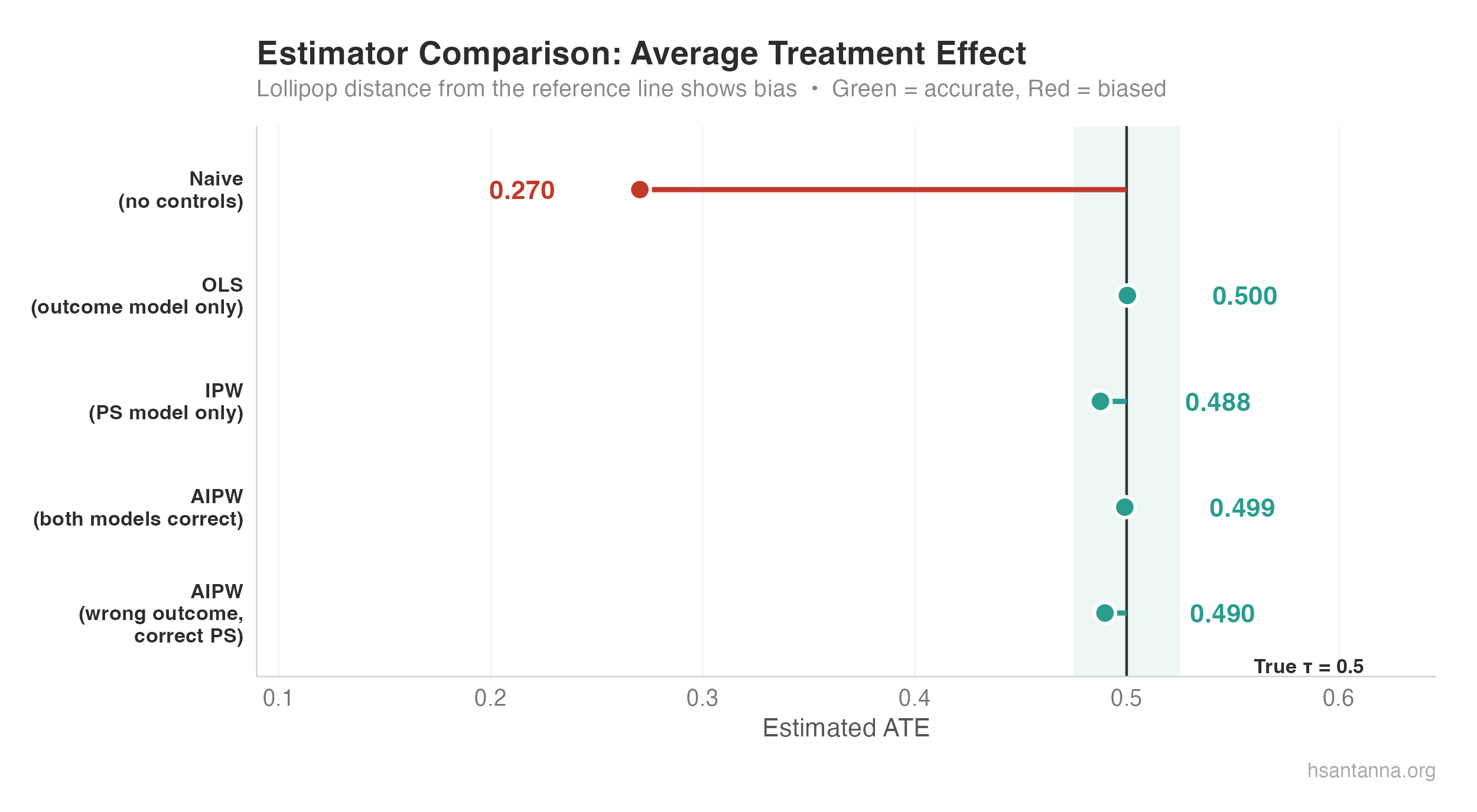
The lollipop chart makes the story clear: the naive estimator (red) is severely biased, while OLS, IPW, and both AIPW variants (green) cluster tightly around the true $\tau = 0.5$.
What comes next?
How do we actually know what is the correct specification for propensity scores? There are many researchers looking out for this answer. Recently, Sant’Anna and Zhao (2020) provided a pathway to use difference-in-differences with doubly robust estimators. And, if you want to go deeper, Kennedy (2022) provides a review of semiparametric methods for doubly robust estimation.