flowchart LR
    D["Job Loss"] -->|direct| Y["Wages"]
    D -->|bad!| X["Occupation"]
    X --> Y
Real-World Application
Wage Scars from Job Loss (NLSY79)
This application demonstrates the bad controls problem using real data from the National Longitudinal Survey of Youth 1979 (NLSY79). The question: how much do wages fall after involuntary job loss?
The setting
Workers who lose their jobs often suffer persistent wage scars — lower wages that persist even years after re-employment. A natural approach is to estimate the wage scar using DiD, comparing separated workers to those who were never separated.
But there’s a catch: job loss also changes occupation. Workers who lose jobs in high-paying occupations frequently end up in lower-paying ones. Occupation is a classic bad control:
- You want to condition on occupation to make parallel trends more plausible (workers in similar occupations have similar wage trends)
- But occupation is causally affected by job loss (the treatment shifts it)
The data
The nlsy_wagescars dataset is a balanced panel of 3,776 individuals from the NLSY79, observed over 9 periods (1984–1993). Treatment is the year of first involuntary job separation.
library(badcontrols)
library(pte)
library(ggplot2)
library(dplyr)

data(nlsy_wagescars)

cat("Panel:", nrow(nlsy_wagescars), "obs,",
    length(unique(nlsy_wagescars$id)), "individuals,",
    length(unique(nlsy_wagescars$period)), "periods\n")

cat("Treatment groups:\n")
g_tab <- table(nlsy_wagescars$G[!duplicated(nlsy_wagescars$id)])
print(g_tab)
Panel: 33984 obs, 3776 individuals, 9 periods
Treatment groups:
0 3 4 5 6 7 8 9
2703 117 106 116 96 209 210 219Occupation changes after job loss
First, let’s verify that occupation is indeed a bad control — that job loss causally shifts it:
occ_means <- nlsy_wagescars |>
  mutate(Group = ifelse(G > 0, "Separated", "Never-Separated")) |>
  group_by(Group, period) |>
  summarize(mean_occ = mean(occ_group), .groups = "drop")

ggplot(occ_means, aes(x = period, y = mean_occ, color = Group)) +
  geom_line(linewidth = 1.2) +
  geom_point(size = 3) +
  geom_vline(xintercept = 2.5, linetype = "dashed", alpha = 0.5) +
  annotate("text", x = 2.7, y = max(occ_means$mean_occ),
           label = "Earliest\nseparation", hjust = 0, size = 3.5) +
  labs(
    title = "Occupation shifts after job loss",
    subtitle = "Mean occupation group (higher = lower-skill occupations)",
    x = "Period", y = "Mean occupation group", color = ""
  ) +
  theme_minimal(base_size = 14) +
  theme(legend.position = "bottom")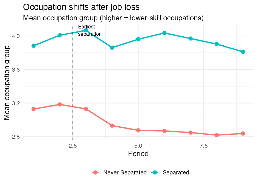
Separated workers are in higher-numbered (lower-skill) occupation groups, and the gap between the two groups widens after separation begins (period 3). This confirms that occupation is affected by treatment — conditioning on it post-separation would absorb part of the wage scar.
Setup
We prepare the auxiliary variable \(W\) (lagged outcome at period 1) for the Covariate Unconfoundedness assumption:
W_df <- nlsy_wagescars |>
  filter(period == 1) |>
  select(id, W = lwage)

panel <- nlsy_wagescars |>
  left_join(W_df, by = "id")
Comparing estimators
Method 0: Naive DiD (no covariates)
res0 <- pte_default(
  yname = "lwage", gname = "G", tname = "period", idname = "id",
  data = panel, d_outcome = TRUE, est_method = "reg"
)
att0 <- extract_att(res0)
cat("ATT:", round(att0$att, 4), " (SE:", round(att0$se, 4), ")\n")
ATT: -0.113 (SE: 0.022 )Method 1: Include occupation directly (bad control)
This conditions on post-separation occupation via regression adjustment. It absorbs the indirect effect through occupation downgrading.
res1 <- pte_default(
  yname = "lwage", gname = "G", tname = "period", idname = "id",
  data = panel, d_outcome = TRUE,
  d_covs_formula = ~occ_group, est_method = "reg"
)
att1 <- extract_att(res1)
cat("ATT:", round(att1$att, 4), " (SE:", round(att1$se, 4), ")\n")
ATT: -0.113 (SE: 0.03 )Method 2: Pre-treatment covariates only
res2 <- pte_default(
  yname = "lwage", gname = "G", tname = "period", idname = "id",
  data = panel, d_outcome = TRUE,
  xformla = ~afqtscore + female + black + hgc, est_method = "reg"
)
att2 <- extract_att(res2)
cat("ATT:", round(att2$att, 4), " (SE:", round(att2$se, 4), ")\n")
ATT: -0.09 (SE: 0.03 )Method 3: Imputation (our proposal)
Imputes counterfactual occupation \(X_t(0)\) — what occupation would have been without job loss — then runs DiD.
res3 <- bc_att_gt(
  yname = "lwage", gname = "G", tname = "period", idname = "id",
  data = panel,
  bad_control_formula = ~occ_group,
  xformla = ~afqtscore + female + black + hgc + W,
  est_method = "imputation",
  lagged_outcome_cov = FALSE
)
att3 <- extract_att(res3)
cat("ATT:", round(att3$att, 4), " (SE:", round(att3$se, 4), ")\n")
ATT: -0.082 (SE: 0.002 )Method 4: Doubly Robust ML (our proposal)
Adds a random forest propensity score correction for double robustness.
res4 <- bc_att_gt(
  yname = "lwage", gname = "G", tname = "period", idname = "id",
  data = panel,
  bad_control_formula = ~occ_group,
  xformla = ~afqtscore + female + black + hgc + W,
  est_method = "dr_ml",
  lagged_outcome_cov = FALSE
)
att4 <- extract_att(res4)
cat("ATT:", round(att4$att, 4), " (SE:", round(att4$se, 4), ")\n")
ATT: -0.081 (SE: 0.028 )Results
| Method | ATT | SE | CI Lower | CI Upper |
|---|---|---|---|---|
| Naive DiD (no covariates) | -0.1130 | 0.0220 | -0.1561 | -0.0699 |
| Include occ (bad control) | -0.1130 | 0.0300 | -0.1718 | -0.0542 |
| Pre-treatment covariates only | -0.0900 | 0.0300 | -0.1488 | -0.0312 |
| Imputation (proposed) | -0.0820 | 0.0020 | -0.0859 | -0.0781 |
| DR/ML (proposed) | -0.0810 | 0.0280 | -0.1359 | -0.0261 |
Interpretation
ImportantThe bad control matters
The naive DiD and bad control approaches estimate a wage scar of about 11% (exp(-0.113) - 1). Our imputation and DR/ML methods estimate about 8%.
The 3 percentage point difference is the indirect effect of job loss operating through occupation downgrading. Conditioning on post-separation occupation masks this channel.
The total wage scar from job loss has two components:
- Direct effect (~8%): lower wages even within the same occupation
- Indirect effect (~3%): job loss pushes workers into lower-paying occupations
Standard approaches that include occupation as a control only recover the direct effect. Our methods recover the total wage scar by imputing what occupation would have been without job loss.
Data access
The nlsy_wagescars dataset is included in the badcontrols package:
library(badcontrols)
data(nlsy_wagescars)
For the full theoretical treatment, see Caetano, Callaway, Payne, and Sant’Anna (2024).