Quick Start to Doubly Robust Estimators

Here, I will provide a simple explanation of doubly robust estimators using R’s tidyverse. This post is heavily inspired by Matheus Facure’s Causal Inference for the Brave and True. There you can find comprehensive tutorials of many causal inference models in Python.

In a first introduction to causal inference, we learn about linear estimators and propensity score weighting methods to estimate the average treatment effect conditional on covariates.

However, covariates are the main source of confounding in causal inference settings, so we should ask: which method should we use? In fact, we can combine both to achieve consistent estimation even when one of the models is misspecified.

Setting up the data

#

Let us imagine we are investigating the causal relationship between income and a government training program in which individuals may or may not participate.

First, we create a very simple static “labor market”. Assume 10,000 workers for whom we observe two variables, X1 and X2.

library(tidyverse)
library(fixest)

set.seed(123)

n <- 10000

# Generate covariates
X1 <- rnorm(n)
X2 <- rnorm(n)

For the sake of simplicity, X1 and X2 are standard normal distributions. We can assume there is a function that maps these draws to real-world data variables — for example, education and work experience.

Treatment assignment

#

Let us now create a treatment variable. In several cases dealing with real-world data, where there is no randomized experiment, assignment to treatment is actually correlated with certain variables in a functional form we may not know.

The key identifying assumption in this exercise is unconfoundedness (also called selection on observables): conditional on X1 and X2, treatment assignment is independent of potential outcomes:

This means that, after conditioning on the covariates, there are no remaining unobserved factors that simultaneously affect both treatment and outcomes. We also require overlap: $0 < P(D = 1 \mid X) < 1$, ensuring that every type of individual has a positive probability of being treated or untreated.

# Generate treatment via logistic model
ps_true <- plogis(-1 - 0.5 * X1 - 0.5 * X2)
treat <- rbinom(n, 1, ps_true)

The naive ATE

#

tau <- 0.5

df <- tibble(
  id = 1:n,
  X1 = X1,
  X2 = X2,
  treat = treat,
  Y = tau * treat + 0.25 * X1 + 0.25 * X2 + rnorm(n, 0, 0.5)
)

naive_ATE <- df |>
  group_by(treat) |>
  summarize(meanY = mean(Y)) |>
  summarize(ATE = diff(meanY)) |>
  pull()

naive_ATE
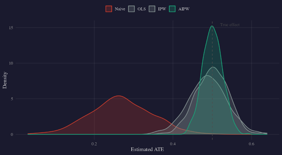
#> [1] 0.2863138

The true treatment effect is $\tau = 0.5$. The naive ATE is biased downward by nearly half. Terrible estimates.

The correct linear model

#

correct_ols <- feols(Y ~ treat + X1 + X2, data = df)
#> treat: 0.5118

We found 0.51 — right on target. So as long as we know the true specification, OLS works.

The propensity score approach

#

ps_model <- feglm(treat ~ X1 + X2, data = df, family = binomial)

df <- df |>
  mutate(
    ps = predict(ps_model, type = "response"),
    weight = ifelse(treat == 1, 1 / ps, 1 / (1 - ps))
  )

Y1 <- sum(df$Y[df$treat == 1] * df$weight[df$treat == 1]) / nrow(df)
Y0 <- sum(df$Y[df$treat == 0] * df$weight[df$treat == 0]) / nrow(df)

correct_PS <- Y1 - Y0
#> [1] 0.5085938

We invert the propensity scores: heavier weights on rarity. A treated observation that looks like a control is more valuable than otherwise. The estimate of 0.508 is very close.

The star of the show: Doubly Robust

#

The main idea: even if we misspecify either the propensity score model or the outcome model (but not both), we still obtain consistent estimates when combining them.

The Augmented Inverse Probability Weighting (AIPW) estimator, due to Robins, Rotnitzky, and Zhao (1994), is:

mu1_model <- feols(Y ~ X1 + X2, data = df |> filter(treat == 1))
mu0_model <- feols(Y ~ X1 + X2, data = df |> filter(treat == 0))

df <- df |>
  mutate(
    mu1_hat = predict(mu1_model, newdata = df),
    mu0_hat = predict(mu0_model, newdata = df)
  )

aipw_1 <- mean(df$treat * (df$Y - df$mu1_hat) / df$ps + df$mu1_hat)
aipw_0 <- mean((1 - df$treat) * (df$Y - df$mu0_hat) / (1 - df$ps) + df$mu0_hat)

DR_ATE <- aipw_1 - aipw_0
#> [1] 0.5118

Excellent — right on target.

Why does it work?

#

Case 1: Outcome model is correct, propensity score is wrong. Both terms have $Y_i - \hat{\mu}_d(X_i)$. If the outcome model is correct, $\mathbb{E}[Y_i - \hat{\mu}_d(X_i) \mid X_i] = 0$ — the propensity score component vanishes.

Case 2: Propensity score is correct, outcome model is wrong. Rearranging isolates $\hat{\mu}_d(X_i)$ paired with $D_i - \hat{P}(X_i)$, which is zero in expectation when the propensity score is correctly specified.

Demonstration with an intentionally misspecified outcome model:

mu1_wrong <- feols(Y ~ 1, data = df |> filter(treat == 1))
mu0_wrong <- feols(Y ~ 1, data = df |> filter(treat == 0))

aipw_misspec_1 <- mean(df$treat * (df$Y - df$mu1_wrong_hat) / df$ps + df$mu1_wrong_hat)
aipw_misspec_0 <- mean((1 - df$treat) * (df$Y - df$mu0_wrong_hat) / (1 - df$ps) + df$mu0_wrong_hat)

DR_misspec <- aipw_misspec_1 - aipw_misspec_0
#> [1] 0.5086

Even with an intercept-only outcome model, AIPW still delivers 0.51 — the correct propensity score carries the identification.

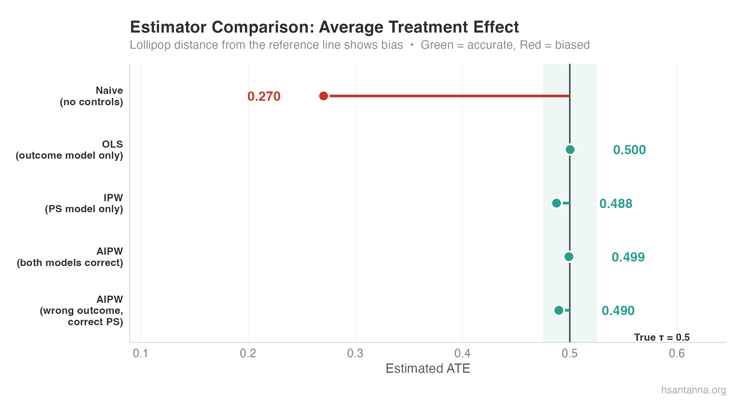
The naive estimator (red) is severely biased. OLS, IPW, and both AIPW variants (green) cluster tightly around the true $\tau = 0.5$.

What comes next?

#

How do we know the correct specification for propensity scores? Sant’Anna and Zhao (2020) provide a pathway to use difference-in-differences with doubly robust estimators. Kennedy (2022) reviews semiparametric methods for doubly robust estimation.