
The EM algorithm is a powerful iterative method for finding maximum likelihood estimates in statistical models with “latent variables” or missing data. It was first proposed by Dempster, Laird, and Rubin (1977) and has since been a common tool in machine learning models.
The core idea is to iteratively alternate between two steps until convergence:
- Expectation (E) step: Estimate the missing data given the observed data and current parameter estimates.
- Maximization (M) step: Update the parameters to maximize the likelihood, treating the estimated missing data as if it were observed.
Eventually (hopefully) the algorithm converges. This is particularly useful for Gaussian mixture models.
A labor market with hidden types#
Say we observe labor market data with log wages and we suspect it is composed of two types of workers: low types and high types. We do not observe the worker type — only the social identifier and their payment.
library(tidyverse)

set.seed(123)
n <- 10000
true_means <- c(2, 3)
true_sds <- c(0.5, 0.5)
true_weights <- c(0.6, 0.4)

lmarket <- tibble(
  worker_id = 1:n,
  type = c(rep(1, n * true_weights[1]), rep(2, n * true_weights[2])),
  log_wage = c(
    rnorm(n * true_weights[1], true_means[1], true_sds[1]),
    rnorm(n * true_weights[2], true_means[2], true_sds[2])
  )
) |>
  mutate(log_wage = log_wage - min(log_wage) + 1)
We can formally write this mixture as:
$$f(w_i; \mu, \sigma, \pi) = \sum^2_{k = 1} \pi_k \mathcal{N}(w_i; \mu_k, \sigma_k)$$The histogram#
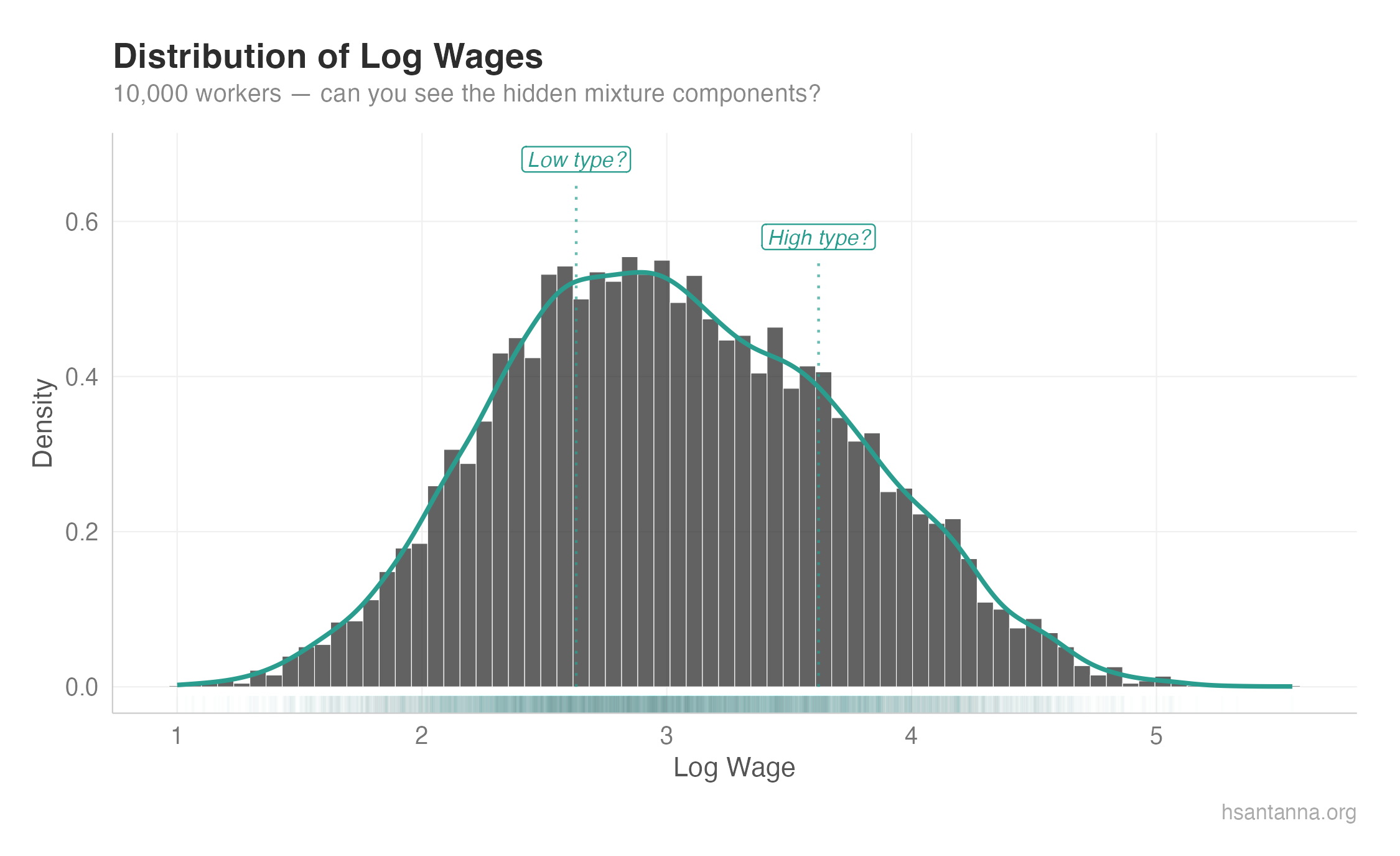
Notice how we can barely see the mixture components. In real-world data, wages are all over the place the same way. There must be “hidden” distributions blended together. So how do we extract them?
The EM algorithm#
The first step is to guess the initial moments and priors using k-means.
initial_guess <- kmeans(lmarket$log_wage, centers = 2, nstart = 25)$cluster

mu1 <- mean(lmarket$log_wage[initial_guess == 1])
mu2 <- mean(lmarket$log_wage[initial_guess == 2])
sigma1 <- sd(lmarket$log_wage[initial_guess == 1])
sigma2 <- sd(lmarket$log_wage[initial_guess == 2])
pi1 <- mean(initial_guess == 1)
pi2 <- mean(initial_guess == 2)
The observed-data log-likelihood is:
$$\ell = \sum_i \log \left( \sum_k \pi_k \mathcal{N}(w_i; \mu_k, \sigma_k) \right)$$Note the log of the sum — this is what makes direct maximization difficult and motivates EM.
sum_finite <- function(x) sum(x[is.finite(x)])

L <- c(-Inf, sum(log(pi1 * dnorm(lmarket$log_wage, mu1, sigma1) +
                      pi2 * dnorm(lmarket$log_wage, mu2, sigma2))))

current_iter <- 2
max_iter <- 500

while (abs(L[current_iter] - L[current_iter - 1]) >= 1e-8 && current_iter < max_iter) {
  # E step
  comp1 <- pi1 * dnorm(lmarket$log_wage, mu1, sigma1)
  comp2 <- pi2 * dnorm(lmarket$log_wage, mu2, sigma2)
  comp_sum <- comp1 + comp2

  p1 <- comp1 / comp_sum
  p2 <- comp2 / comp_sum

  # M step
  pi1 <- sum_finite(p1) / length(lmarket$log_wage)
  pi2 <- sum_finite(p2) / length(lmarket$log_wage)
  mu1 <- sum_finite(p1 * lmarket$log_wage) / sum_finite(p1)
  mu2 <- sum_finite(p2 * lmarket$log_wage) / sum_finite(p2)
  sigma1 <- sqrt(sum_finite(p1 * (lmarket$log_wage - mu1)^2) / sum_finite(p1))
  sigma2 <- sqrt(sum_finite(p2 * (lmarket$log_wage - mu2)^2) / sum_finite(p2))

  current_iter <- current_iter + 1
  L[current_iter] <- sum(log(pi1 * dnorm(lmarket$log_wage, mu1, sigma1) +
                              pi2 * dnorm(lmarket$log_wage, mu2, sigma2)))
}
The EM algorithm guarantees monotone ascent: $\ell(\theta^{(t+1)}) \geq \ell(\theta^{(t)})$.
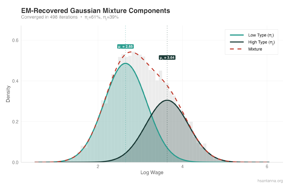
Results#
Converged in 498 iterations
  Component 1: mu = 2.654, sigma = 0.498, pi = 0.614
  Component 2: mu = 3.641, sigma = 0.502, pi = 0.386
The estimated parameters are very close to the true values.

The two Gaussian components (teal and dark teal) are clearly separated, and their weighted sum (dashed red) closely matches the empirical density.
What about model selection?#
What if we assume 3 worker types instead of 2? You’ll get a tiny third component ($\hat{\pi}_3 \approx 0.018$) that the algorithm struggles to fit — a clear sign of overfitting. AIC and BIC penalize complexity and help balance fit against overfitting.