So, what is bunching?

Here I explain the basic concepts of bunching as a causal inference method. Full replication code is on GitHub.

library(tidyverse)
library(ggdag)
library(AER)

set.seed(20240804)

Constructing the data

#

We need a data generating process where an unobserved confounder $\eta$ affects both the treatment (cigarettes) and the outcome (birth weight), while a covariate (education) is also observed.

n <- 5000

educ <- sample(6:16, n, replace = TRUE)
eta <- rnorm(n)

cigs_star <- 20 - 1.5 * educ + 5 * eta + rnorm(n, 0, 3)
cigs <- pmax(0, round(cigs_star))
bw <- 3000 - 20 * cigs + 15 * educ - 10 * eta + rnorm(n, 0, 100)

data <- tibble(bw = bw, cigs = cigs, educ = educ)

The key feature: $\eta$ directly affects both cigs_star (smoking propensity) and bw (birth weight). This is the unobserved confounder that will bias naive estimates.

The naive approach

#

Imagine you’re interested in the causal effect of smoking on birth weights. You observe a covariate, mom’s education, and you control for it:

naive_model <- lm(bw ~ cigs + educ, data = data)
summary(naive_model)

Notice something weird? Can you say that for every cigarette smoked per day, the baby loses about 40 grams?

Probably not.

#

The hint is in the educ coefficient — wrong-signed or insignificant. It implies babies are worse off (or no better off) as we increase the mom’s education level.

What if there’s an unobserved $\eta$ that influences both birth weights and the propensity to smoke?

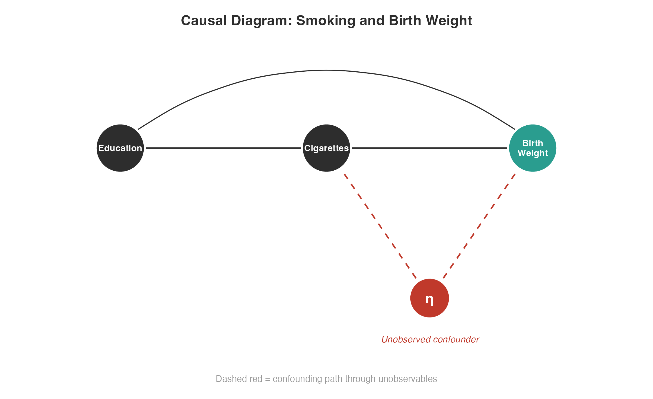
There are 3 causal paths to birth weights: a direct path from education, another from $\eta$, and another where cigarettes act as a mediator variable. Not only are we incorrectly estimating the cigarettes-birth weights relationship, we’re probably messing with the education path too.

Enter bunching

#

The key assumption: there is a proxy relationship between smoking and covariates. Individuals have a propensity to smoke, like a utility function. Some maximize this utility by smoking heavily. Others are very averse — they would pay not to smoke. And then there are the marginally inclined — they would smoke given a chance but are slightly better off not smoking.

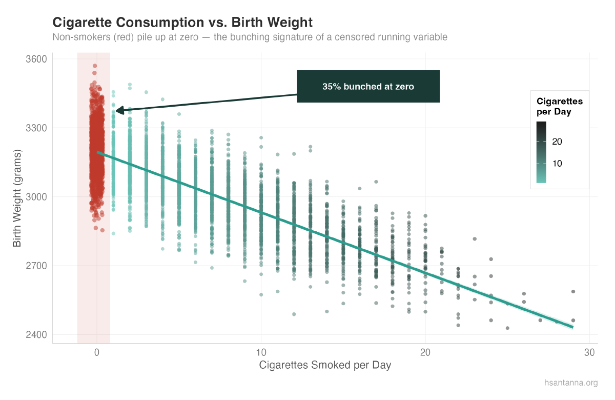
We partially observe this mechanism. We only see individuals who are positively inclined to smoke — there is no negative cigarette consumption.

Notice the linear relationship until we hit zero — then a bunching pattern of birth weights. The puzzle: why are there so many data points accumulated at zero?

The running variable

#

There’s a variable we don’t observe that “runs” continuously through zero and accepts negative values. If we could capture this variable, we could isolate the cigarettes–birth weight relationship without the confounding $\eta$.

Formally:

$X$ is a proxy for $X^*$, the running variable that is continuous in zero and can assume negative values.

Assuming linearity:

Combining:

The trick: we impute $\mathbb{E}(X^* \mid X^* \leq 0, Z)\cdot\mathbb{1}(X = 0)$ as a proxy for when $X$ becomes 0 — we now “observe” negative cigarette values. This accounts for the unobservable confounder.

The Tobit approach

#

Since our data is censored at zero, we assume normality of the latent error: $\eta \sim \mathcal{N}(0, \sigma^2)$. A Tobit model recovers the truncated conditional expectation:

tobit_model <- tobit(cigs ~ educ, data = data, left = 0)

sigma_hat <- tobit_model$scale
xb <- predict(tobit_model, type = "lp")

mills <- dnorm(-xb / sigma_hat) / pnorm(-xb / sigma_hat)
trunc_exp <- xb - sigma_hat * mills

data <- data |>
  mutate(cf_imput = ifelse(cigs == 0, trunc_exp, 0))

The key step is the inverse Mills ratio correction. The linear predictor $Z’\hat{\pi}$ alone is not $\mathbb{E}(X^* \mid X^* \leq 0, Z)$ — we must account for the truncation.

cf_model <- lm(bw ~ cigs + educ + cf_imput, data = data)

The coefficient on cigs should now be close to the true value of $\beta = -20$. Compare with the naive OLS, which was biased toward $-40$.

Where is the randomness?

#

Causal experiments usually rely on random shocks. But here individuals bunched at zero simply because they cannot smoke less than zero. We need randomness to ensure unobservables are not affecting the treatment effect — in bunching, we exploit the bunched values to reach the unobservable confounder and ultimately control for it.

Further reading

#

For a deeper overview, see Bertanha, McCallum, and Seegert (2024) and the original Caetano (2015).